Python and pyROOT Tutorial
Outline
This tutorial serves as a generic introduction to python and a brief introduction to the high-energy physics analysis package
"pyROOT". It is designed to take about 2 hours to read through and run the examples. That is just enough time to get started with python, have a feel for how the language works and be able to write and run simple analysis programs. I've not attempted to cover everything including coding best practices. Please note also that as most of the high energy physics software runs in python version 2, this tutorial uses the python version 2 syntax.
The source code for the tutorials is available here:
The root manual and reference guide:
https://root.cern/manual/
https://root.cern/
Please email itsupport@physics.ox.ac.uk with any errors.
1) What is python?
From the python website:
Python is an interpreted, object-oriented, high-level programming language with dynamic semantics. Its high-level built in data structures, combined with dynamic typing and dynamic binding, make it very attractive for Rapid Application Development, as well as for use as a scripting or glue language to connect existing components together. Python's simple, easy to learn syntax emphasizes readability and therefore reduces the cost of program maintenance. Python supports modules and packages, which encourages program modularity and code reuse. The Python interpreter and the extensive standard library are available in source or binary form without charge for all major platforms, and can be freely distributed.
Often, developers fall in love with Python because of the increased productivity it provides. Since there is no compilation step, the edit-test-debug cycle is incredibly fast. Debugging Python programs is easy: a bug or bad input will never cause a segmentation fault. Instead, when the interpreter discovers an error, it raises an exception. When the program doesn't catch the exception, the interpreter prints a stack trace. A source level debugger allows inspection of local and global variables, evaluation of arbitrary expressions, setting breakpoints, stepping through the code a line at a time, and so on. The debugger is written in Python itself, testifying to Python's introspective power. On the other hand, often the quickest way to debug a program is to add a few print statements to the source: the fast edit-test-debug cycle makes this simple approach very effective.
Breaking this down:
- High level - Programmers can write code that is agnostic to the underlying hardware or operating system
- Built in data structures - Python has a great number of built in types. In addition to the usual ints and floats the built in string class for example is extremely powerful. As well as this, the syntax for creating, loops and lists and other collection objects is more natural than for older languages. Developers can use their available time more wisely by dealing with high level abstractions rather than low-level types.
- Python is "interpreted" - Meaning no compilation step is needed.
[**] Python can and is often used in place of more traditional shell and perl scripts since it has almost as powerful string parsing abilities but much more straightforward syntax.
[**] In addition, the type of an object is determined when the script runs. The amount of typing is much reduced (no more "const int* blah = getBlah();"). This can allow rapid-prototyping, i.e. writing a function/class/program to perform a desired task quickly. It does, however, introduce a class of bugs that strongly typed languages do not automatically suffer from.
[**] Programs written entirely in python also run more slowly than well-written compiled code. However, if this turns out to be a problem there ways to re-write only parts of the program in C/C++. This is exactly how "pyROOT" (discussed below) interfaces to ROOT. - Python supports modules - Because python is quite an easy and well used open language there are thousands of people who have written extensions or "modules" to perform certain tasks well. With python is is always worth a quick google to see whether someone has written something to do pretty much what you want. Because python is also quite readable and distributed and run from it's source code, it is usually quite easy to see exactly what a library is doing.
2) Python vs c++
Normally, start by using python unless you need to use C++ for some reason. Those reasons include:
- Someone has already done >75% of the work in C++.
- I don't know any python (lets fix that).
- I have profiled my python code and realised that doing "X" operation is really slow, I have already re-written the python to be faster and it is still a problem.
- I am writing a non-linear program and the compile-time error-trapping and type checking that one gets for free with a compiler is important to me to catch edge-case bugs.
Consider two programs, one in C++ and one in python
//A C++ Program called hello.cpp #include "iostream" int main(int argc, char** argv) { std::cout<<"Hello World" << std::endl; return 0; }
demo@pplxint8 > g++ hello.cpp -o hello demo@pplxint8 > ./hello Hello World
#A program written in python #!/usr/bin/python print "Hello World"
demo@pplxint8 > python ./hello.py
There is often a lot less to type when writing a python program or script. There are fewer steps to remember and get wrong (write and run vs write, compile and run). Perhaps most important when it comes to finding errors is the clarity of python code.
3) Running the python interpreter
Python's main power comes with how easy it is to get something that works. Part of that power is the rapid prototyping that is made possible by the interpreter. Python comes with a native interpreter that can be used simply by running:
demo@pplxint8 > python
We can quit with Ctrl+D.
However, the basic interpreter lacks a few features. A better one is "ipython".
Python has a few built in types, such as your usual ints, floats. It also naively supports quite complex strings and string modification functions. Lets start with something simple to demonstrate using the the variable "aString" to store the text "hello world":
The interpreter also offers standard "shell-like" features such as tab completion and history - try tab completion by typing "aSt" in the example above and then tab before pressing enter. In addition, the history buffer can be scrolled by pressing up/down arrows or searched with 'Ctrl+R', starting to type the command, e.g. the first part, "hell" of "hello" in the example above and then Ctrl+R to scroll through the matches.
To create runnable reusable code, you should write your code to a '.py' file. After prototyping with "ipython", you can copy the inputs that you made into the console out to a .py file using the save magic function. The syntax is 'save {file-name} {line-numbers}'.
> ipython In [1]:print 'hello world' In [2]:save 'mySession' 0-1 In [3]:Ctrl+D
> cat mySession.py # coding: utf-8
print 'hello world'
You can then re-run your old code with:
If you are running on a machine integrated with a batch system such as pplxint8/9, you can scale up and out your python session onto the batch nodes. This would be achieved by adding "#!/usr/bin/python as the first line in your saved "mysession.py" file and then running qsub mysession.py.
Python types often come with their own documentation. This can be accessed using help(type) or even help(variable) from the command line. Just to view all of the symbols defined by the type, dir(type/variable) will also work.
4) Basic Syntax
Python uses white-space to delineate code blocks or 'scopes' Anything indented to the same degree is considered to be part of the same scope. Variables defined within an indented scope can persist after the end of the scope except for in new class and function scopes. Some statements require that a new scope is opened after they are used - we will introduce some of these later.
Comments in python are denoted with a hash ('#') symbol. The text between the hash symbol and the end of the current line is not treated as code. Instead it is used to provide a hint to people reading your code as to what it does. As a rule of thumb, about 1/3 of the text in your python programs should normally be in comments.
Variable types (eg int, float) are rarely explicitly specified in python except when they are first defined. Python will decide for you what type a variable is. We say that the variables in python are not strongly typed (however the values are). To create a new variable, just write a name that you want to refer to it by and then use the assign (=) operator and give it a value. E.g to assign the value '2' to the identifier 'myNumber', simply write 'mynumber = 2'. You can then use myNumber anywhere in your code and the interpreter will treat every occurrence just as if you had directly written the number '2'. Unlike some languages, no type needs to be specified and no special characters are needed to indicate that you want the variable to be expanded to it's value.
5) Built-in Types and simple functions
Python has a range of built in types and has powerful introspection features. In python it is rare to specify the type of a variable directly. Instead, just let python decide.
Python function calls, similar to other languages, use parenthesis "()" to indicate the function. If the function takes arguments, the arguments go into the parenthesis separated by commas.
The type() function can be used to determine the type at run-time. Some examples are below.
In [33]: iX=1
In [34]: type(iX) Out[34]: int
In [35]: fY=1.0
In [36]: type(fY) Out[36]: float
In [37]: sZ='string'
In [38]: type(sZ) Out[38]: str
In [39]: uUniExample=u'string'
In [40]: type(uUniExample) Out[40]: unicode
In [41]: lListExample=[1,'a']
In [42]: type(lListExample) Out[42]: list
In [43]: dDict={'a', 'b', 4}
In [44]: type(dDict) Out[44]: dict
In [43]: bBool=True
In [44]: type(bBool) Out[44]: bool
It is also easy change the type of a variable just by reassigning a new variable of a different type, e.g.
Debugging tip: This ability to change the type of a variable at run-time is a powerful feature, but it can also be dangerous and its misuse has in the past actually doubled the amount of time we spent working on one project. When the type() function is scattered into your debugging statements together with a convention of storing the variable type somewhere in the variable name, one can often spot errors caused by passing the wrong type of variable to a function more quickly. When the type should absolutely not change, I choose to use the first letter of the variable name to indicate its type - see code lines 33-44 above for examples.
6) Containers
Lists
Python's most basic conventional container is a list. A list may contain mixed parameter types and may be nested. Elements within the list can be accessed by using the integer corresponding to that element's position in the list, starting from '0'.
We can also re-assign elements of the list, and add to the list with the append() member function. The len() function gives the length of containers.
The "append" function illustrates "member functions". Member functions of classes modules can be accessed by giving the class instance name or module name post-fixed by a dot and then the member function or variable: e.g. myString.append('value').
You can use either double quotes or single quotes to enclose a string. You can use this fact to include quotes in your string, e.g.
print 'and they said "python strings are very powerful"'
More on strings
In python, a string is really a sequence container. It supports the "len()" and index "[]" operations like the list above.
In [12]: sMyString='0123456789a'
In [13]: len(sMyString) Out[13]: 11
In [14]: sMyString[2] Out[14]: '2'
What do you think the following code will do?
Though the variables are not strongly typed, the values are. The operator (*) is a duplicate operator for the string.
Dictionary
The python dictionary class is more powerful than the list type. You can use any type as the index, not just an integer. In the example below, we emulate the above list using a dict then add on an element using a string type as the index.
In [15]: dMyDict={ 0:1, 1: 2, 2: ['a', 'b', 'c'], 3: 'Last one'}
In [16]: dMyDict Out[16]: {0: 1, 1: 2, 2: ['a', 'b', 'c'], 3: 'Last one'}
In [17]: len(dMyDict) Out[17]: 4
In [18]: dMyDict[4]='e'
In [29]: print dMyDict {0: 1, 1: 2, 2: ['a', 'b', 'c'], 3: 'Last one', 4: 'e'}
In [20]: len(dMyDict) Out[20]: 5
In [21]: dMyDict['arbitrary_type']='another_type'
In [22]: dMyDict Out[22]: {0: 1, 1: 2, 2: ['a', 'b', 'c'], 3: 'END', 4: 'e', 'arbitrary_type': 'another_type'}
7) Loops and conditionals
"if" conditional
The syntax for a python if statement is:
Loops
Loops in python can be controlled by the for and while loops. The in keyword can be used to generate a sequence of values directly from the list.
Here is an example of both for and while loops:
###1-Control demo 1 in the source code attached### l=['a','b','c'] count=0 while count < 3: print l[count], ' is l from while loop' count=count+1
for val in l: print val, ' is l from for loop'
The continue statement tells the code to jump straight to the next iteration of the loop and stop executing any more code in this iteration. The break statement jumps straight out of the loop and executes no further code in the for or while loop. Notice also I have introduced the 'not' keyword, which negates the expression it prefixes. I have also introduced the rather standard shorthand for count=count+1, namely count+=1
8) File I/O
A common problem is that a text file containing data formatted in a certain way is given to you as input data. Your job will need to parse and analyse this datafile.
Now see demo3 in the attached source code
9) Writing functions
It is advisable to constantly review your code and divide it up into re-usable functions where possible. The def keyword allows you to define and write functions. Use the def keyword followed by the name for your function, followed by any arguments in parenthesis and finishing with a colon (:). Functions can also take default arguments. The default arguments are not used if an overriding parameter is passed to the function when it is called. You can also return one (or more) values using the return keyword.
#!/usr/bin/python ###Function demo 1#### #First define the function that will be used def myFirstFunction(myParam1, myParam2='default'): #Indent 4 spaces print myParam1 #Check whether the second parameter is the default one or not if 'default' == myParam2: #Indent 4 spaces print 'I was not passed a second parameter' else: print 'I was passed a second parameter, it was: ', myParam2 #Return a string saying everything went well #Note, convention is to return the integer '0' if the function behaved as expected #or a non-zero integer if there was an error. return 'OK'
# no indent # the first non-indented (or commented) line without the def or class keyword is the # entry point of the code print 'About to run my function' myFirstFunction('I am running in a function!!') retval=myFirstFunction('Passing Another Parameter','"this text"') print '"myFirstFunction" returned "', retval, '"'
Now see demo2 in the attached source code
10) Keywords
So far we have covered most of what is needed to write a simple program, and it is beyond the scope of this introduction to cover all python reserved words. However, a list of the python reserved keywords is given here for completeness so that the reader can look up these online.
The following identifiers are used as reserved words, or keywords of the language, and cannot be used as ordinary identifiers. They must be spelled exactly as written here:
Note that although the identifier as can be used as part of the syntax of import statements, it is not currently a reserved word.
In some future version of Python, the identifiers as and None will both become keywords.
11) Modules and passing command line arguments to python
Python has a lot of built-in functionality, but that is nothing compared to what exists in the extensions or 'modules' than have been written for python. I cannot tell you how to use them all, or even what ones are available. Try googling what you want to do, and usually you will find a module to do it. Once you know which module you want, fire up the (i)python interpreter and type import module-name, where module-name is the name of the module e.g. "sys" or "os". We can install extra python modules on the particle Linux systems as required. You can also install your own personal copy in a python "virtual environment", which is often more appropriate. See the next main section for details.
The modules often come with their own documentation. This can be accessed using help(module-name) from the command line. Just to view all of the symbols defined by the module, dir(module-name) will also work. Usually googling "python module-name" is just as good or better! A notable exception to all that is when running pyROOT (i.e. importing ROOT into python).
To use some feature of the module, give the module name followed by the function, class or variable that the module provides with a dot in between.
The sys module
A heavily used module is the 'sys' module, which is most often used to pass information from the calling shell to python and vice versa.
#!/usr/bin/python ###Module demo 2### import sys #get the number of parameters passed to the python program argc=len(sys.argv) #Loop over the arguments passed to the program and print them out. #Note that the first argument is always the name of the running program. for arg in sys.argv: print arg
#Exit with a status of '0' to indicate to the shell that the python program ran OK. sys.exit(0)
You should also familiarise yourself with the "os" module, which is also used a lot.
Now see demo4 in the attached source code
12) Extending python with additional modules and running newer python versions
Python has a feature called virtual environments. This allows you to build on system versions of python to do the following:
- Add additional modules that are not already installed on the system
- Run newer versions of modules than the system provides
- Run a newer version of python than the system provides
- Have several different projects with potentially conflicting python module requirements
To create a virtualenv called myVirtualEnv, do the following.
Every time you wish to use the virtualenv in the future, run just the following.
At this point, you will notice your prompt change to indicate you are running in a virtualenv. You can install new python modules into the virtual environment. Lets now look for and install a package to help with plotting in numpy
I can now run some numpy code
More information on numpy and pyplot can be found here
http://matplotlib.org/users/pyplot_tutorial.html
Running newer versions of python in your virtualenv
On most university and research lab systems, IT will be able to install a new version of python if requested, so I wont cover that here. To make use of these versions of python all you need is the path to the new python version. For example in physics.
Running python3 virtualenvs
For python 3, virtualenvs have been replaced. Some of the early versions of python 3 had various issues, but from python 3.4.5 things seem very smooth with the new tool "pyvenv". It is very similar to virtualenvs.
To set up a python 3.4.5 pyvenv:
To load it again for re-use:
Multiple simultaneous environments (advanced)
You can layer multiple virtualenvs on top of each other. Lets say for example you want to use the system packages, and a standard set of additional packages maintained by your experiment followed by a few updates you are testing yourself. To prepare such an environment, there is the python package called "envplus".
An example below shows how to import the virtualenv we prepared above for another user so that numpy is pre-installed.
In a current writable directory:
Following that, its just the same as before
13) pyROOT - for PP students only
Up to now, this tutorial has been quite generic. This part is for particle physics students.
Some helpful chap has wrapped up the entirety of ROOT into a python module. Since python syntax is more natural than C++ and the python interpreter does not suffer from as many bugs and problems with non-standard syntax as the 'CINT' interpreter, I recommend using pyROOT instead of CINT when you are starting any program from scratch. People may suggest that python is slower than C++. It is, but that statement applies to compiled C++ not CINT, for the most part it doesn't matter and also you need to know C++ well to make it very fast. At the end of the day, any really slow parts of your code can be re-written in C(++) if absolutely necessary. Remember two generalizations about C++ and general execution times.
1) The average C++ software engineer writes 6 lines of useful, fully tested and debugged code per day.
2) 80% of the CPU time will be spent on 20% of your code even after you have optimised the slow parts.
Lets begin by setting up root. To use pyROOT, the C++ libraries must be on your PYTHONPATH. This is set up automatically by the most recent Oxford set-up scripts.
In the case of pyROOT a deliberate decision was made by the developers not to import all of the symbol names when import is run. Only after the symbol is first used is it available to the interpreter (e.g. via tab-complete or help()).
Lets now import the ROOT module into root and use it to draw a simple histogram.
In [1]: import ROOT In [2]: ROOT.gROOT.Reset() In [3]: dir(ROOT) Out[3]: ['PyConfig', '__doc__', '__file__', '__name__', 'gROOT', 'keeppolling', 'module']
In [4]: x=TH1F()
In [5]: dir(ROOT) Out[5]: ['AddressOf', 'MakeNullPointer', 'PyConfig', 'PyGUIThread', 'SetMemoryPolicy', 'SetOwnership', 'SetSignalPolicy', 'TH1F', 'Template', '__doc__', '__file__', '__name__', 'gInterpreter', 'gROOT', 'gSystem', 'kMemoryHeuristics', 'kMemoryStrict', 'kSignalFast', 'kSignalSafe', 'keeppolling', 'module', 'std']
Debugging tip: If you are changing the version of python (sometimes implicit when altering your root version) you may want to eithe re-create your ipython profile (rm -r ~/.ipython; ipython profile create default) or run ROOT.gROOT.Reset() to allow the graphics to be displayed.
To use root in the ipython interpreter and create, fill and draw a basic histogram:
In [1]: import ROOT, time In [1]: ROOT.gROOT.Reset() In [2]: hist=ROOT.TH1F("theName","theTitle;xlabel;ylab",100,0,100) In [3]: hist.Fill(50) Out[3]: 51
In [4]: hist.Fill(50) Out[4]: 51
In [5]: hist.Fill(55) Out[5]: 56
In [6]: hist.Fill(45) Out[6]: 46
In [7]: hist.Fill(47) Out[7]: 48
In [8]: hist.Fill(52) Out[8]: 53
In [9]: hist.Fill(52) Out[9]: 53
In [10]: hist.Draw() Info in <TCanvas::MakeDefCanvas>: created default TCanvas with name c1 In [11]: save 'rootHist' 1-10 In [12]: ctrl+D pplxint9.physics.ox.ac.uk%> echo '#Sleep for 10 secs as a way to view the histogram before the program exits'>> rootHist.py pplxint9.physics.ox.ac.uk%> echo 'time.sleep(10)'>> rootHist.py pplxint9.physics.ox.ac.uk%> python rootHist.py
You can view the contents of rootHist.py using an editor like "emacs".
To fill an ntuple/Tree
import ROOT ROOT.gROOT.Reset() # create a TNtuple ntuple = ROOT.TNtuple("ntuple","ntuple","x:y:signal") #store a reference to a heavily used class member function for efficiency ntupleFill = ntuple.Fill
# generate 'signal' and 'background' distributions for i in range(10000): # throw a signal event centred at (1,1) ntupleFill(ROOT.gRandom.Gaus(1,1), # x ROOT.gRandom.Gaus(1,1), # y 1) # signal
# throw a background event centred at (-1,-1) ntupleFill(ROOT.gRandom.Gaus(-1,1), # x ROOT.gRandom.Gaus(-1,1), # y 0) # background ntuple.Draw("y")
Instead of launching the script from the Linux command line, it is possible to run the script from within the "ipython" interpreter and keep all your variables so that you can continue to work.
Also, a feature of the root module means that the ntuple and the new canvas appears in the ROOT name-space for you to continue using it in your program too.
You can also find your objects again using the TBrowser.
The GUI that pops up has a number of pseudo-directories to look in. Open the one that says 'root' in the left pane and navigate to ROOT Memory-->ntuple. You can double click on your histograms to draw them from here.
By right-clicking on the name of your ntuple (in this case just 'ntuple') and navigating to 'Start Viewer', you can drag and drop the variables to draw as a histogram or apply as a cut. Drag signal into the box marked with scissors and x onto the 'x' box. Click the purple graph icon to Draw. You may have to create the canvas first. You can do that from the new TBrowser - See the "Command" box in figure 1.

Figure 1: Editing a cut and creating a canvas from the TBrowser
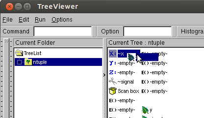
Figure 2: Making a new canvas from the Browser
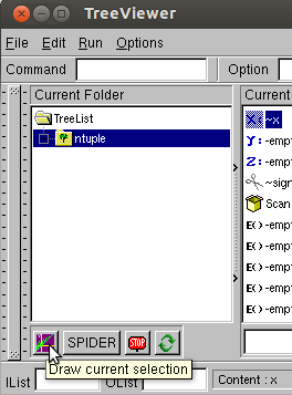
Figure 3: The draw current selection box
Filling an ntuple
The attached source code contains a workable demonstration of working with ROOT ntuples, covering:
Now work through demo 5 in the attached source code
Garbage collection (specific to ROOT but not specific to pyROOT)
Normally, garbage collection is classed as an advanced concept, however in my experience most of the annoyance of ROOT in general was to do with seemingly random crashes. Most of these were actually due to the object I was using disappearing at various point in the program. This was due to misunderstanding ROOT's object ownership model, which functions as a poor-mans garbage collection. This happens outside of python.
Root objects are not persistent. They are owned by the directory they "exist" within. In this case the histogram is actually owned by the canvas (which is itself a directory in ROOT), but the ntuple only contains a reference to it. TDirectory and TPad classes and derived classes count as directories in this model.
One way to rescue the situation, if you want the histogram to outlive the canvas you can make a copy:
or you can remove the histogram from the pad before you close it
Chapter 8 of the ROOT manual details more on object ownership.
14) Additional Resources:
Official python tutorial
Google python tutorial complete with videos. Videos cover the simple topics in quite a lot of depth.
pyroot at cern
15) Optimization tricks
The most important thing is to do good Physics, fast computer code comes later. However, since I am in charge of looking after the batch systems, I have a vested interest in your code not crippling the entire computing system. This exercise also gives more practice importing and using someone elses modules (profiler and stats).
There is one place where python is very slow and there is an easy fix. That is when running code in a loop. This section will demonstrate that slowdown and give a solution to the problem.
Generally only optimize where it is needed. Even the world experts can't guess where this will be needed 100% of the time.
To find what is taking the time, a little tool called cProfile exists. Run this example program to see how it works. Spend the time looking only at optimizing the functions that are taking time. I have two functions, foo and bar. I want to know which to optimize. From the output, it looks like bar needs optimizing.
import cProfile #Define 3 functions that do something. In this case the content of the functions is not the relevant thing.
def add(a): a+=1 def bar(): print 'y' for x in range(2000000): add(x)
def foo(): a=0 for i in range(10): print i for j in range(100000): a+=j #calling bar from within foo bar()
#The point of this exercise is the profiler. Declare a new profiler called 'fooprof' which will immediately run the foo() function like this: cProfile.run('foo()','fooprof') #To output the results of the profiler, we need pstats import pstats pf = pstats.Stats('fooprof') #Print out the sorted stats print pf.sort_stats(-1).print_stats()
Common cause of python slowdowns
There is a quick way to speed up python code to play a trick when repeatedly using a class member function. Store the class member function function in a variable and use that to make the function call.
In the example which follows, the class member function is adder.add and it is stored in a variable adderadd. Have a play with commenting in and out the various add calls in the foo() function and re-running the code. Note how the time taken to look up the class member function reference is counted against the time taken to run the foo function, rather than against the function that is being looked-up (add).
Note, this section is about optimizing a function being called repeatedly in a loop. The function could have been doing anything, it just so happends I chose addition. This section is not about optimizing addition.
import cProfile
class adder: def add(self, x): x+=1
def add(x): x+=1
def foo(): print 'y'
myadder=adder()
#take a reference to the class member function adderadd=myadder.add
for x in range(200000):
#Fastest is to use a function without the class add(x)
#slowest is to make python look up the class and function every time myadder.add(x)
#Almost the fastest, python no longer needs to look up where the class member function 'is' each time as the result of that lookup is cached (in adderadd). adderadd(x)
cProfile.run('foo()','fooprof') import pstats p = pstats.Stats('fooprof') print p.sort_stats(-1).print_stats()
We learn from this that by creating a local reference to a class member function for our innermost loops, we can speed up python dramatically.
For more tips, see https://wiki.python.org/moin/PythonSpeed/PerformanceTips.
#SLOW for i in range(10000): myclass.foo()
#FAST mcfoo=myclass.foo for i in range(10000): mcfoo()
All of this is available in demo 6 in the attached source code
16) Ipython notebooks
Ipython notebooks allows you to run python in a web-browser and save your sessions. You can connect from the interactive machine on which you are running and any graphics will pop up on your X display (i.e. not in the browser).
As with all web applications, anyone connecting to the application can do whatever you can do.
To avoid this, there is some additional set-up to do, which you should do if you want to make it hard for anyone connected to the machine to delete all of your files (for example). So set a password on the browser. This is probably safe enough for use on the interactive machines if you connect from the firefox webbrowser that is installed on the machine on which you run the notebook.
Make a little python script that does this:
##############makepass.py############
#!/bin/env python
from IPython.lib import passwd
print passwd()
#################################
Create an ipython profile to include the settings for the notebook.
> ipython profile create default
You may need to remove the existing ipython configuration that you have with
>rm -fr ~/.ipython
Add the following line to $HOME/.config/ipython/profile_default/ipython_notebook_config.py:
c.NotebookApp.password = u'longoutputstring'
Where longoutputstring is the whole string returned to you when you ran the little makepass.py script above.
Be absolutely sure nobody can read this file:
chmod og-rwx $HOME/.config/ipython/profile_default/ipython_notebook_config.py
You can then run the notebook (on pplxint8) with:
jupyter
An improvement on python notebooks is 'jupyter'. I found this difficult to install, but works in python3. To use jupyter:
Contact:
The goal of this introduction was to teach the minimum you need to get up and running. This is not a formal training, but a means to get you into doing Physics with pyROOT. I am always interested in keeping this page live with hints, tips and techniques that you find useful and may help out others. Please email suggestions to itsupport@physics.ox.ac.uk.
Categories: ppunix | pyROOT | python | virtual Python